Assignment 10

Scientific Plotting and Data Visualization with PGFPlots

Objective

In this assignment, you will produce a one page extended abstract in LaTeX and include one plot created with PGFPlots. The plot must read data from data.txt.

Instructions

Folder Structure

Create a main folder named Assignment10.

Steps

1. Create the data file

Inside Assignment10, create a file named data.txt.
Copy and paste the data below into data.txt.

0.000 1.000
0.314 1.309
0.628 1.588
0.942 1.809
1.256 1.951
1.570 2.000
1.884 1.951
2.198 1.809
2.512 1.589
2.826 1.310
3.140 1.002
3.454 0.692
3.768 0.412
4.082 0.191
4.396 0.049
4.710 0.000
5.024 0.048
5.338 0.190
5.652 0.410
5.966 0.690
6.280 0.997

2. Create the LaTeX file

Inside Assignment10, create a file named main.tex.
Copy and paste the code below into main.tex.

\documentclass[a4paper,11pt]{article}

\usepackage[utf8]{inputenc}
\usepackage{geometry}
\usepackage{pgfplots}
\usepackage{titlesec}
\usepackage{tikz}

\pgfplotsset{compat=newest}
\geometry{left=2cm,right=2cm,top=2cm,bottom=2cm}

\title{\textbf{Extended Abstract: Data Based Visualization of an Offset Sinusoidal Sensor Signal}}
\author{Your Name \\
MECH0291 Computer Programming}
\date{}

\begin{document}
\maketitle
\vspace{-0.6cm}

\section*{Abstract}
Sinusoidal signals appear in many engineering systems such as rotating machinery, vibration sensors, and alternating current measurements.
This short study demonstrates a clean workflow where raw measurements stored in a plain text file are plotted directly inside a \LaTeX\ document using \texttt{pgfplots}.
The dataset in \texttt{data.txt} represents an offset sinusoidal sensor output over one period, where the offset models a common hardware bias.

\section*{Methodology and Discussion}
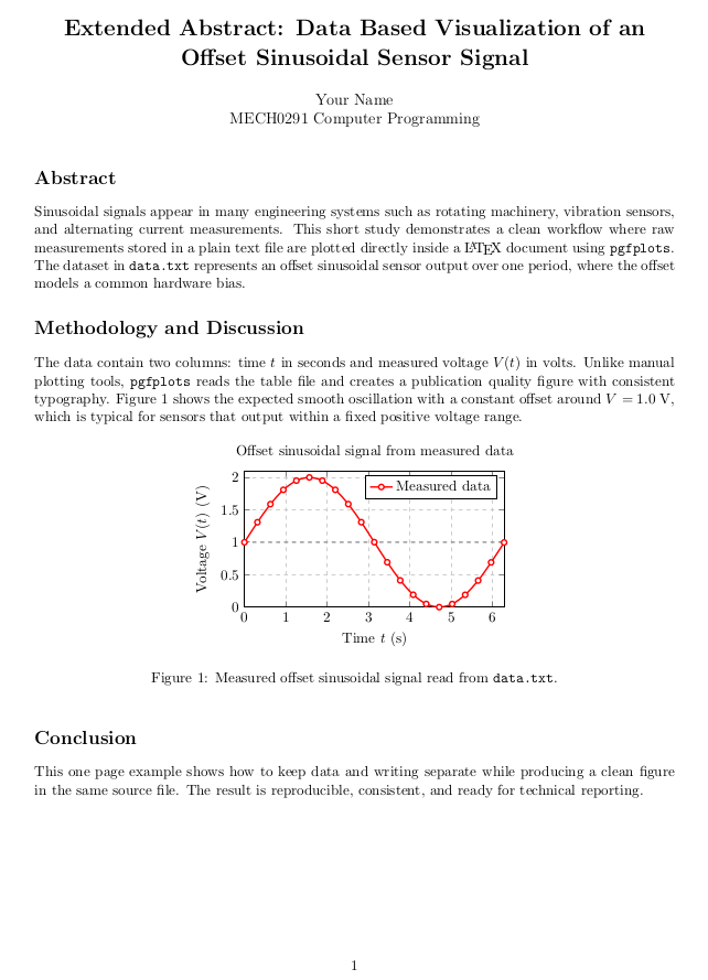
The data contain two columns: time $t$ in seconds and measured voltage $V(t)$ in volts.
Unlike manual plotting tools, \texttt{pgfplots} reads the table file and creates a publication quality figure with consistent typography.
Figure 1 shows the expected smooth oscillation with a constant offset around $V=1.0$ V, which is typical for sensors that output within a fixed positive voltage range.

\begin{figure}[ht]
    \centering
    \begin{tikzpicture}
        \begin{axis}[
            width=8.5cm, height=5.2cm,
            title={Offset sinusoidal signal from measured data},
            xlabel={Time $t$ (s)},
            ylabel={Voltage $V(t)$ (V)},
            grid=major,
            grid style={dashed, gray!40},
            xmin=0, xmax=6.3,
            ymin=0, ymax=2.1,
            legend pos=north east,
            thick
        ]
        \addplot[
            color=red,
            mark=*,
            mark options={fill=white},
            line width=1.2pt,
            smooth
        ] table [x index=0, y index=1] {data.txt};
        \addlegendentry{Measured data}

        \addplot[gray, dashed, forget plot] coordinates {(0,1.0) (6.3,1.0)};
        \end{axis}
    \end{tikzpicture}
    \caption{Measured offset sinusoidal signal read from \texttt{data.txt}.}
\end{figure}

\section*{Conclusion}
This one page example shows how to keep data and writing separate while producing a clean figure in the same source file.
The result is reproducible, consistent, and ready for technical reporting.

\end{document}

3. Compile

Open a terminal and go into the Assignment10 folder.
Run:

pdflatex main.tex

4. Verify the Output:

- Ensure that the generated `main.pdf` matches the required structure as in the figure below.

5. Clean up

Delete every file except main.tex, data.txt, and main.pdf.
You can run:

rm main.aux main.log

6. Final folder check

Your final folder must contain only these files:

Assignment10/
|__data.txt
|__main.tex
|__main.pdf

7. Submit

Submit the Assignment10 folder (with only those three files).

Submit your Assignment 10

Run this command while you are inside the Assignment10 folder:

submitAssignment.sh